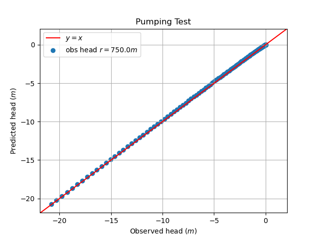
Scatterplot of drawdowns from pairs of observation well during the numerical pumping tests modeling. The predicted heads was obtained using 1D GRF solution.

Topics, Skills and Tools Used

Formulation

GRF model

To validate the results of the simulations, for example for the construction of a benchmark, it is normal to use analytical solutions that describe the process in which the numerical model will simulate. For pumping test modeling, the Theis solution (1935) is normally used for this purpose. The modeling of this project is characterized by having a domain with two dimensions where the water flow is unidimensional (along the x axis), for the simplest case of an aquifer with constant thickness (benchmark). However, Theis solution describes the drawdown of hydraulic loads through the radial flow of groundwater. Thus, it was necessary to use an analytical solution that describes this one-dimensional flow and, therefore, can describe the data obtained by the numerical model in order to establish the benchmark for the problem. This equation used is the solution of Generalized Radial Flow Model (GRF), developed by Baker (1988).

The GRF was created with the objective of solving the problem of describing the drawdown of hydraulic loads due to pumping in fractured media. The specific problem is choose the appropriate geometry of a fracture system in which underground flow occurs. This solution was developed by generalizing the dimensional flow to non-integral values while maintaining the assumptions of radial flow and aquifer homogeneity. In this way, the GRF is able to describe the drop in hydraulic loads in various forms used (geometry) in pumping tests (Baker, 1988). The assumptions of this model are:

• Groundwater flow is radial and n-dimensional in a homogeneous and isotropic medium with hydraulic conductivity Kf and specific storage Ssf .
• Darcy's law applies to the entire system.
• Water withdrawal from the system is through an n-dimensional sphere with radius rw and storage capacity Sw.

The following GRF analytical solution (Baker, 1988) is an equation that has been generalized from Theis (1935) solution:

$$h(r, t) = \frac{Q_0 r^{2 \nu}}{4 \pi^{1 - \nu} K_f b^{3 - n}} \Gamma(-\nu, u) \qquad \nu<1 $$

With:

$$\nu = 1 - \frac{n}{2} $$

$$u = \frac{S_{sf} r^2}{4 K_f t} $$

$$\Gamma(s, x) = \int_{x}^{\infty} t^{s - 1} e^{-t} \,dx $$

Where:

• h(r, t) is the function of describing the hydraulic loads for position r at time t for the system.
• Q0 is the constant pump rate.
• r is radial distance from the pumping well.
• n is the system dimension.
• b is the extent of the flow region.
• t being the time

For the problem of this project, as already mentioned, the flow of water in the porous medium occurs in a one-dimensional way, therefore, n = 1. As a result, we have the following form of the GRF model solution, used in the data analysis:

$$h(r, t) = \frac{Q_0 r}{2 \sqrt{\pi} K_f b^2} (\frac{e^{-u}}{\sqrt{u}} - \sqrt{\pi} {erfc} \sqrt{u})$$

Where erfc is the complementary error function. Note that for the case of n = 2 the GRF model solution becomes the Theis solution. The GRF solution was applied through the use of the Python Anaflow library for the implementation of the benchmark.

Numerical model governing equation

A confined aquifer model, isotropic and with homogeneous K was created. The governing equation of groundwater flow in a confined aquifer is governed primarily by the hydraulic head variable. The groundwater flow equation for this case is derived from the principles of conservation of mass and momentum within continuum mechanics. The description of fluid movement used was the Eulerian one in which it considers its observation in a control volume through which this fluid enters and leaves

The groundwater flow was considered in a non-deformable porous medium. In this way the only way for the water to flow is through the empty spaces. The porosity (n) is given by the ratio of these voids to the total volume of the medium. As it was considered that the medium is not deformable and, therefore, the empty spaces variable is considered constant throughout the simulation. With this we have that the mass balance equation (fluid) in a static porous medium is given by:

$$\frac{\partial n \rho}{\partial t} + \nabla (n \rho v) = Q_{\rho}$$

Where ρ is the fluid density [kg/m³], t the time [s], v the velocity vector [m/s] and Qρ the groundwater entry term into the system [kg/m³s]. Considering water as an incompressible fluid and, therefore, with constant density (“outside” the derivation) this implies that ρ = ρ0. Dividing the above equation by ρ0 we have:

$$\frac{\partial n}{\partial t} + \nabla (n v) = \frac{Q_{\rho}}{\rho_0}$$

The Storativity (S) is a concept that encompasses the change of n over time. The relationship between the change in n and the hydraulic head (h in m) with time is linear with a change ratio factor S:

$$\frac{\partial n}{\partial t} = S \frac{\partial h}{\partial t}$$

We also have the linear relationship that explains the groundwater flow due to a hydraulic head gradient in space in porous media, with K as a proportion factor. This relationship is given by the Darcy equation:

$$n v = q = -K \nabla h$$

Combining the balance equation (second equation) with the constitutive equations (third and fourth equations in this governing equation section), results in the governing equation for groundwater flow in confined aquifers used in the simulation:

$$S \frac{\partial h}{\partial t} - \nabla (K \nabla h) = Q$$

Results

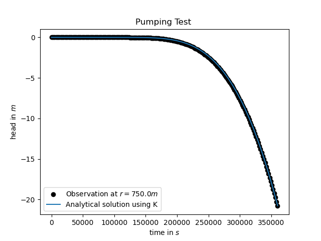
Drawdown curve obtained of the conducted experiment. Observed head was got from numerical modeling (black dots).
Predicted heads was obtained from the 1D GRF model equation (blue curve).

Scatterplot of drawdowns from pairs of observation well during the numerical pumping tests modeling.
The predicted heads was obtained using 1D GRF solution.

References

Barker, J.A., 1988. A generalized radial flow model for hydraulic tests in fractured rock, Water Resources Research, vol. 24, no. 10, pp. 1796-1804.

Theis, C. V. (1935), The relation between lowering the piezometric surface and the rate and duration of discharge of a well using ground water storage, Eos Trans. AGU, 16, 519–524.